



Google Cloud Dataflow: Guides, Pricing, Cost Optimization

For many teams operating in Google Cloud environments, Google Cloud Dataflow becomes a critical component for large-scale data processing and streaming workloads. Meantime, its operational behavior, cost dynamics, and scaling mechanics are often misunderstood.
Without understanding how pipelines scale, how resources are allocated, and how job execution impacts latency and spend, teams risk inefficiencies and unexpected costs.
In this article, we’ll cover these aspects and more – in short, everything you need to get started the right way.
Key Takeaways
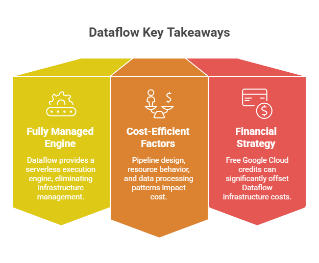
> Google Cloud Dataflow provides a fully managed serverless execution engine for batch and streaming data pipelines, eliminating infrastructure management overhead.
> To stay cost-efficient with the Dataflow usage, you have to keep in mind several factors: pipeline design, resource behavior, data processing patterns, etc.
> Beyond technical optimization, financial strategy matters. Leveraging free Google Cloud credits through Spendbase can significantly offset Dataflow infrastructure costs.
What Is Google Cloud Dataflow
Google Cloud Dataflow is Google Cloud’s fully managed data processing service built on Apache Beam. It enables unified programming for both batch and streaming analytics using a single execution model.
Compared to traditional data processing flows, Google Cloud Dataflow provides a fundamental shift: instead of managing infrastructure, teams can significantly reduce operational overhead and focus on pipeline logic.
Here’s the difference it makes: in traditional models, there are many manual processes involved – in particular, a great amount of time and effort is taken by these ones:
- Cluster provisioning;
- Capacity planning;
- Node lifecycle management;
- Scaling orchestration.
Dataflow replaces them efficiently with dynamic resource allocation, automatic autoscaling, platform-managed workers, and other capabilities (see more details in the table below). This way, infrastructure complexity is significantly reduced.
| Traditional Data Processing Model | Google Cloud Dataflow Model |
| Manual cluster provisioning | Fully managed infrastructure |
| Capacity planning required | Dynamic resource allocation |
| Node lifecycle management | Worker management handled by platform |
| Scaling requires intervention | Scaling handled automatically |
| Fixed resource sizing | Automatic autoscaling |
| Idle resources during low load | Resources allocated on demand |
| Infrastructure-first operations | Pipeline-first operations |
| Manual failure recovery | Built-in retries & fault tolerance |
| Performance tied to cluster size | Performance tied to pipeline design |
| Scaling events may cause disruption | Online, non-disruptive scaling |
With this in mind, Google Cloud Dataflow has several key highlights:
> Serverless architecture. No cluster provisioning or infrastructure management, compute resources are fully abstracted and platform-managed.
> Automatic scaling. Workers are dynamically allocated based on workload characteristics such as throughput, backlog, and latency.
> Deep integration with the Google Cloud ecosystem. Native connectivity with services like Pub/Sub, BigQuery, Cloud Storage, and Vertex AI simplifies pipeline design and data movement.
> Adaptive, dynamic execution model. Dataflow pipelines are not static compute jobs – they continuously react to input throughput, backlog pressure, processing latency, resource utilization, and other factors to automatically adjust execution and maintain high performance.
Most importantly, Dataflow functions as a real-time data intelligence platform to help organizations maximize the value of continuously moving data. See its capabilities and most common use cases below.
| The Functional Scope of Dataflow | ||
| Dimension | What Dataflow Handles | Typical Scenarios |
| Batch Processing | Large-scale dataset transformations | Data warehouse preparation, historical analytics |
| Stream Processing | Low-latency event pipelines | Real-time metrics, fraud detection, IoT telemetry |
| Autoscaling | Dynamic worker allocation | Variable workloads, bursty pipelines |
| Fault Tolerance | Automatic retries & checkpointing | Long-running pipelines |
| Resource Optimization | Worker lifecycle management | Cost-efficient scaling |
| Unified Execution | Same logic for batch & stream | Simplified pipeline development |
See how much you can save on your stack
Pick your team’s tools!
Click to select one or more tools.


What’s your company size?
Just click to select.
What’s your business email?
We'll send you calculations right away
The email is flying to your inbox!
Beyond discounts, you may qualify for up to $100K in AWS credits.

How Google Cloud Dataflow Works
In practice, Dataflow executes pipelines defined using Apache Beam. The pipeline itself defines the logical data processing flow, while Dataflow is responsible for executing that logic at scale.

As illustrated above, a typical Apache Beam pipeline goes as follows:
External System → Data Source. Applications, IoT devices, databases, or SaaS platforms generate raw events, logs, or transactional data.
Pub/Sub → Ingestion. Pub/Sub receives and buffers streaming data. This way, it decouples producers from processing systems and ensures reliable, scalable message delivery.
Dataflow → Processing. After that, Google Cloud Dataflow subscribes to Pub/Sub and processes data in parallel across worker VMs. It applies transformations (filtering, aggregation, enrichment) and automatically scales based on workload. Then, processed data is written to BigQuery.
BigQuery → Analytics Storage. In BigQuery, the data is stored in a scalable columnar format optimized for SQL-based analytics.
Looker and Data Visualization. Looker connects to BigQuery to provide dashboards and reports – on system performance, analytical takeaways (trends, segmentation, KPI analysis), executive insights, etc.
Key Google Cloud Dataflow Capabilities (And How To Maximize Them)
#1: Fully Managed Execution
Dataflow is a fully managed service that owns the entire compute lifecycle, from worker VM allocation to automatic deletion when the job completes or is cancelled.
However, keep in mind this often misinterpreted fact (based on our observations): while Dataflow is a fully managed service, “fully managed” does not mean fully automatic decision-making.
What it means: Dataflow takes ownership of infrastructure provisioning, scaling, and runtime reliability. You, in turn, still remain responsible for pipeline design, architecture choices, and, in particular, cost control.
| What Dataflow Handles Automatically | What You Still Define / Manage |
| Provisions and deletes worker VMs | Pipeline logic (Apache Beam code) |
| Distributes work across workers | Data sources and destinations |
| Autoscaling based on workload (CPU, memory, backlog, throughput) | Worker type selection (machine sizing) |
| Replaces failed workers | Pipeline configuration parameters |
| Retries failed tasks | Data modeling and schema design |
| Dynamically rebalances workload | Optimization of transforms and joins |
| Manages checkpointing and state (streaming jobs) | Business logic and windowing strategy |
| Applies infrastructure patches and maintenance | Cost monitoring and budget control |
| Shuts down resources when job completes | IAM permissions and access policies |
#2: Dynamic Autoscaling
Google Cloud Dataflow proved itself as a mature, execution-aware scaling model. What’s important, Dataflow evaluates pipeline-level signals (see the table below listing them). Thanks to this, scaling decisions are directly tied to processing health and latency SLOs (unlike traditional autoscaling that reacts to CPU or memory thresholds).
This makes scaling decisions directly tied to processing health and latency SLOs, not indirect infrastructure metrics.
The Functional Scaling Signals in Google Cloud Dataflow | |
| Signal category | What It Measures |
| Stage throughput | Records processed per stage per unit time |
| Backlog growth | Pending elements waiting for processing |
| Watermark progression (Streaming) | Event-time advancement |
| Task completion rates | Work item execution velocity |
| System lag | Event time vs processing time gap |
| Worker utilization (Contextualized) | CPU & memory interpreted with pipeline state |
| Parallelism saturation | Whether additional workers increase throughput |
| Hot key / data skew signals | Uneven key distribution across workers |
| Straggler detection | Outlier long-running tasks |
| Bundle processing time Distribution | Execution time variance across bundles |
| Dynamic work rebalancing signals | Ability to split and redistribute work |
| State growth & checkpoint patterns | Stateful stage memory and checkpoint trends |
| Backpressure propagation | Downstream stage congestion |
Practically, thanks to these signals, Google Cloud Dataflow autoscaling is able to deliver three critical advantages:
- Predictable latency under variable load, which is especially important for streaming workloads with strict timeliness requirements;
- Improved cost-performance ratio (capacity expands only when pipeline pressure justifies it and contracts when demand stabilizes).
- Reduced operational overhead with minimal need for manual tuning, reactive scaling policies, or capacity forecasting.
Meantime, note this: to fully leverage this capability, the pipeline must be architected for horizontal scalability from the outset (since Dataflow can only parallelize what the pipeline logically allows it to parallelize).
#3: Parallelized & Optimized Processing
WithGoogle Cloud Dataflow, you do not need to manually shard datasets or coordinate worker communication – the system handles task distribution and dynamic work rebalancing internally.
As illustrated in the diagram, you can see how Google Cloud Dataflow enables fully parallelized and runtime-optimized processing: by automatically decomposing high-level transforms into parallel execution stages, optimizing the execution graph (including shuffle boundaries like GroupByKey), and distributing work across workers without manual sharding or coordination.
#4: Fault-Tolerant Design
Another important factor is that Google Cloud Dataflow solves the critical issue distributed workloads struggle with – partial failures (worker crashes, transient network issues, stragglers, infrastructure interruptions, etc.)
How differentiator that makes a difference compared to distributed workloads inherently experience partial failures. Dataflow is designed for resilience. A few aspects that stand out in this domain:
- Automatic worker recovery. If a worker VM crashes or becomes unhealthy, tasks are reassigned and retried automatically without manual intervention.
- Transparent task re-execution. Work items (bundles) can be safely reprocessed. The system manages retries internally, minimizing operational overhead.
- Durable state management (streaming). Stateful processing relies on persistent state backends. Checkpointing mechanisms ensure progress is preserved across failures.
- Exactly-once processing guarantees (where supported). Through checkpointing, idempotent sinks, and coordinated commits, Dataflow maintains strong correctness semantics for streaming pipelines.
- Shuffle and intermediate data durability. Shuffle data is persisted to prevent data loss during worker replacement or scaling events.
- Backpressure-aware recovery. When failures occur, downstream pressure is managed to avoid cascading instability.
- Rolling updates without job disruption. Infrastructure maintenance and worker replacement can occur without stopping the pipeline.
#5: Streaming & Batch Support at Scale
Google Cloud Dataflow supports both batch and streaming workloads within a unified execution model, which is a significant architectural advantage. This allows teams to build pipelines once and run them in batch or streaming without re-architecting core logic.
For real-time use cases, Google Cloud Dataflow provides a specialized streaming execution engine optimized for:
- Event-time processing and watermark management;
- Flexible windowing (fixed, sliding, session windows);
- Late data handling with configurable triggers;
- State management for long-running pipelines;
- Low-latency processing under sustained ingestion loads.
One of the recent feature releases in Google Cloud Dataflow introduced ML enhancements for streaming workloads, including accelerator-aware scaling to improve GPU utilization within a unified framework. See the comparison below.
| Streaming Execution in Google Cloud Dataflow: Comparison | ||
| Standard Streaming Execution | Streaming with GPU-Enabled ML Workflows | |
| Execution Model | Unified Beam-based streaming engine | Same unified streaming engine |
| Primary Focus | Event-driven analytics & ETL | Real-time ML inference & feature processing |
| Compute Infrastructure | CPU-based workers | CPU + optional GPU workers |
| Autoscaling Inputs | Backlog size, throughput, CPU utilization | Backlog, throughput, CPU + GPU utilization |
| Scaling Intelligence | Pipeline-aware autoscaling | Pipeline-aware + accelerator-aware autoscaling |
| State & Windowing | Full support (event-time, watermarks, triggers, durable state) | Same capabilities preserved |
| Fault Tolerance | Automatic retries & checkpoint-backed recovery | Same guarantees preserved |
| Architectural Model | Single execution paradigm | Same execution paradigm with heterogeneous compute |
#6: Flexible Pipeline Development
Google Cloud Dataflow supports multiple development and deployment approaches. Its pipelines can be developed and delivered through:
- Custom pipelines using Apache Beam SDKs – supporting full control over transforms, windowing logic, stateful processing, ML integration, etc.;
- Google Cloud Dataflow templates (Classic & Flex), which package pipelines for reusable and parameterized deployment;
- Google-provided templates for common scenarios (e.g., Pub/Sub to BigQuery, GCS to BigQuery, log processing) to accelerate implementation without custom code;
- Interactive development via JupyterLab notebooks for rapid prototyping and iterative testing.
Based on our observations, you’ll get the greatest value if you treat pipelines as versioned, deployable artifacts: build and validate in Beam, package with Flex Templates, parameterize environments, and integrate into CI/CD. This will ensure cross-environment consistency and prevent configuration drift as teams scale.
#7: Observability & Monitoring
Without execution-aware observability, diagnosing data pipeline issues becomes guesswork. For this reason, Google Cloud Dataflow jobs are easily observable through the Google Cloud Console monitoring interface, which provides the following insights:
- A graphical representation of the pipeline execution graph;
- Stage-level progress tracking;
- Bottleneck and latency identification;
- Worker-level metrics;
- CPU usage and memory profiling;
- System lag and data freshness indicators;
- Autoscaling behavior insights.
Besides, to extend its visibility beyond the execution graph in the console, Google Cloud Dataflow integrates with the broader Google Cloud observability ecosystem. Browse its top integrations below.
| Observability Integrations in Google Cloud Dataflow | |
| Integration | Scope |
| Google Cloud Monitoring | – Custom dashboards – SLO tracking – Alerting |
| Google Cloud Logging | – Detailed execution logs |
| Google Cloud Trace | – Latency tracing across services |
| Error Reporting | – Aggregated runtime error tracking |
| Custom Beam Metrics | – User-defined counters – Distributions- Gauges |
| Cloud Profiler | CPU and memory profiling (supported scenarios) |
| IAM Audit Logs | Access and permission activity logs |
| VPC Flow Logs | Network traffic visibility |
| External metrics export (e.g., Prometheus) | Integration with third-party observability stacks |
Google Cloud Dataflow Pricing Overview
Google Cloud Dataflow pricing is consumption-based and primarily driven by compute resource usage. You pay only for what the job consumes, which is flexible for both steady and bursty workloads.
Its major cost drivers include:
- Worker configuration – machine type, vCPU-to-memory ratio, number of workers;
- Pipeline runtime – continuous execution, job duration, backfills;
- Autoscaling dynamics – minimum worker baseline, max worker limits, scale-down behavior;
- Shuffle & data movement – large joins, windowed aggregations, key skew, cross-region transfers.
See more details in the pricing breakdown below.
Pricing Breakdown: Google Cloud Dataflow | ||
| Pricing Component | Behavior | Price Range |
| vCPU Usage | Charged per worker compute time | $0.056 / vCPU-hour |
| Memory Usage | Billed alongside vCPU | $0.00356 / GiB-hour |
| Shuffle Operations | Charged for data redistribution | $0.011 / GiB processed |
| Streaming Engine Compute | Separate optimized pricing for streaming | $0.071-$0.089 / compute unit-hour |
| Aggregate job cost (hourly) | Combined compute, memory, shuffle | $2-$6 / h (for moderate jobs) |
vCPU Usage (Primary Cost Driver)
Google Cloud Dataflow provisions worker virtual machines to execute your pipeline. You are billed based on the total compute resources consumed across all active workers (specifically, the cumulative virtual CPU hours used during pipeline execution).
These charges are calculated as follows: Number of workers × vCPUs per worker × runtime (in hours).
| vCPU Usage Decision Table for Google Cloud Dataflow | ||
| Scenario | Recommended Strategy | Cost Risks? |
| Simple ETL (batch) | Balanced machine type with autoscaling enabled | Low |
| CPU-intensive transforms (parsing, encryption, ML inference) | Compute-optimized machine types (higher vCPU ratio) | Medium (if overprovisioned |
| Large joins / heavy shuffle | Increase worker count before increasing per-worker vCPU | Medium |
| Stateful streaming | Right-size workers; rely on autoscaling for throughput changes | High (if running 24/7) |
| High-throughput streaming ingestion | Scale horizontally (more workers) instead of vertically | High (compounding runtime cost) |
| Small data, long runtime job | Downsize machine type; avoid idle vCPU hours | Medium (silent waste) |
| Unpredictable burst workloads | Enable autoscaling; set appropriate max worker limits | Controlled if governed |
Memory Usage
In Google Cloud Dataflow, memory is billed separately from CPU. In this area, the ultimate cost depends on three core factors: 1) worker machine type, 2) number of workers, 3) pipeline runtime.
Specifically, you pay based on the RAM capacity of the worker VMs you select. This means you pay for the total memory provisioned across all workers for the duration of the job, regardless of whether the memory is fully utilized. So, if you choose larger machine types, it will increase memory costs even if CPU usage remains moderate.
| Memory Configuration Decision Table for Google Cloud Dataflow | |||
| Scenario | Memory Requirement | Recommended Strategy | Cost Risks? |
| Simple ETL (batch) | Low | Balanced machine type (standard memory ratio) | Low |
| CPU-intensive transforms | Moderate | Compute-optimized (more vCPU, standard RAM) | Medium (if overprovisioned) |
| Large joins / groupByKey | High | Memory-optimized (higher RAM per vCPU) | Medium |
| Stateful streaming | High | Memory-optimized, + Streaming Engine | High (if long-running) |
| Large record processing | Moderate to high | Balanced, scale up only in case of memory pressure | Medium |
| Unpredictable workloads | Moderate | Begin balanced, monitor metrics before scaling | Controlled if monitored |
Shuffle Operations
Unlike CPU and memory costs, shuffle pricing is directly tied to the volume of data moved between workers, not to runtime or machine type.
Ultimately, the cost depends on three core factors: 1) volume of data entering shuffle stages, 2) number of shuffle-heavy transformations, 3) frequency of windowing or aggregation operations (especially in streaming).
From our experience, cost spikes in this domain commonly occur during:
- GroupByKey;
- Aggregations;
- Joins;
- Windowed computations;
- Any transformation that requires data from multiple workers to be reorganized.
| Shuffle Cost Decision Table for Google Cloud Dataflow | |||
| Scenario | Shuffle Intensity | Recommended Strategy | Cost Risks? |
| Simple ETL (batch) | Low | Minimize unnecessary grouping | Low |
| Single aggregation stage | Moderate | Ensure proper key distribution | Medium |
| Large joins | High | Pre-filter data before join, reduce dataset size early | High |
| Wide GroupByKey operations | High | Avoid skewed keys; consider combiners | High |
| Windowed streaming aggregations | High (recurring) | Use appropriate window size, enable Streaming Engine | Very high |
| High-cardinality keys | Moderate to high | Validate partitioning strategy | Medium |
| Unoptimized pipeline with multiple reshuffles | Extremely high | Reduce shuffle stages, redesign transformation logic | Very high |
Streaming Engine Compute
For streaming workloads, Google Cloud Dataflow provides a separate Streaming Engine pricing model. Because streaming pipelines are typically long-running, even moderate compute unit consumption can accumulate significant monthly costs. See more details based on specific scenarios.
| Streaming Engine Cost Decision Table for Google Cloud Dataflow | |||
| Scenario | Streaming Compute Intensity | Recommended Strategy | Cost Risks? |
| Low-volume real-time monitoring | Low | → Enable Streaming Engine → Monitor baseline compute unit use | Low |
| Moderate event-driven analytics | Moderate | → Optimize window size → Reduce state retention | Medium |
| High-throughput ingestion | High | → Scale horizontally first → Set autoscaling limits carefully → Review sustained peak traffic | High |
| Stateful streaming with large windows | High | → Reduce window duration → Implement state TTL policies | High |
| Streaming joins | High | → Pre-filter datasets before joins → Minimize join key skew | High |
| 24/7 production streaming | Continous | → Conduct regular cost reviews → Right-size baseline workers → Remove idle pipelines | Extremely high |
| Unbounded state growth | Extremely high | → Enforce strict state expiration → Redesign unbounded key logic | Critical |
Data Transfer
Network egress is billed under standard Google Cloud networking rules. Costs vary depending on three main aspects: 1) region, 2) cross-region transfer, 3) internet egress.
To understand and calculate your data transfer costs correctly, consider these aspects:
> Costs increase even if CPU usage is low. Network pricing is volume-based, large outputs can be expensive even in lightweight pipelines.
> Export-heavy jobs can cost more than the processing itself. Writing large datasets to external systems often drives network spend.
> Regional misalignment is a common hidden cost driver. Running Dataflow in one region while accessing data in another triggers cross-region fees.
> Cross-region reads can be introduced unintentionally during scaling. Expanding storage or adding new sinks without regional alignment increases costs.
> Internet egress can outpace compute in data-heavy systems. External transfers are typically more expensive than intra-cloud traffic.
| Data Transfer Cost Decision Table for Google Cloud Dataflow | |||
| Scenario | Transfer Level | Recommended Strategy | Cost Risks? |
| Same-region architecture | Low | Keep Dataflow, GCS, BigQuery in same region | Low |
| Multi-region storage access | Moderate | Align pipeline region with storage region | Medium |
| Cross-region writes | High | Avoid inter-region routing unless required | High |
| Internet egress | High | Compress data; reduce output payload size | High |
| Real-time external streaming | Very high | Aggregate/filter before sending externally | Very high |
| Hybrid cloud integration | Moderate to high | Use dedicated networking (VPC peering, VPN) | Medium |
Now, if we consider a realistic scenario with a continuously running Dataflow pipeline using ~10 workers over a full month, the estimated monthly cost would be over $1,600 on average, including all pricing components. See the breakdown below.
Google Cloud Dataflow Cost: Realistic Monthly Cost Scenario | |||
| Pricing Area | Scenario Usage | Pricing Basis | Estimated Monthly Cost |
| vCPU Usage | ~10 workers × 24h × 30 days ≈ 7,200 vCPU-hours | $0.056 per vCPU-hour | $403 |
| Memory Usage | ~10 workers × ~32 GiB × 24h × 30 days ≈ 230,400 GiB-hours | $0.00356 per GiB-hour | $820 |
| Streaming Engine | Moderate streaming workload | $0.071-$0.089 per compute unit-hour | $110 – $160 |
| Shuffle / Data Processing | ~18 TB processed / month | $0.011 per GiB processed | $198 |
| Data Transfer | Limited egress (~300 GB) | $0.05–$0.12 per GB (depending on region) | $15-$36 |
| Total | $1,546-$1,617 | ||
Free virtual cards for non-EU residents
Open in 1 working day, issue 100 virtual cards, and get up to 1.25% cashback.
Get a free account
Common Cost Pitfalls in Google Cloud Dataflow
From our observations, inefficiencies typically stem from pipeline design patterns rather than pricing mechanics.
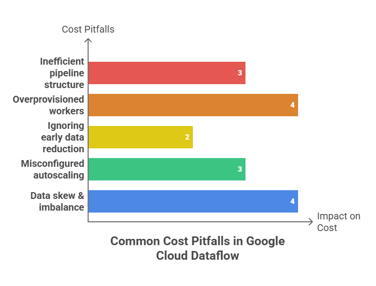
- Inefficient pipeline structure. Poor transform ordering and excessive reshuffling increase compute time and resource usage.
- Overprovisioned workers. Oversized machine types lead to low utilization and continuous cost waste.
- Ignoring early data reduction. Processing unnecessary data inflates shuffle volume, runtime, and worker allocation.
- Misconfigured autoscaling. Improper worker limits or slow scale-down causes sustained over-allocation and cost volatility.
- Data skew & imbalance. Uneven key distribution prolongs execution, thus increasing compute consumption.
Cost Optimization Strategies for Google Cloud Dataflow
Optimizing Google Cloud Dataflow costs requires a layered approach. The framework below separates quick tactical wins from deeper architectural optimizations – check it out.
Quick Wins for Google Cloud Dataflow Cost Optimization | |||
| Strategy | Effort | Savings | Impact Speed |
| Right-size workers | Low | High | Immediate |
| Optimize autoscaling | Medium | High | Fast |
| Reduce shuffle operations | Medium | Very High | Fast |
| Apply early data filtering | Low | Very High | Immediate |
| Use Streaming Engine | Low | Medium–High | Immediate |
| High-Impact Structural Optimizations | |||
| Optimize pipeline topology | High | Very high | Gradual |
| Reduce data volume early | Medium | Very high | Fast |
| Balance parallelism | High | High | Gradual |
| Control autoscaling sensitivity | Medium | High | Fast |
| Continuous pipeline monitoring | Medium | High | Ongoing |
Getting Started With Google Cloud Dataflow
Step 1. Choose the right development approach
Dataflow runs pipelines defined by Apache Beam, but not every workload requires writing custom SDK code. Google Cloud Dataflow offers several options to simplify this process for you:
1 – Templates (with prebuilt pipelines for common integrations (e.g., Pub/Sub & BigQuery);
2 – Job Builder for low-code pipeline creation through a visual interface;
3 – MLTransform (simplifying training and inference workflows);
4 – Apache Beam SDK, offering full customization for advanced pipelines.
With the correct entry path selected, you’ll be able to reduce unnecessary complexity and prevent architectural overengineering from the very start. Below, see a list of recommendations from the official Google Dataflow documentation.
Step 1. Classify workload type
Clarify the following from the very beginning: batch vs. streaming, latency-sensitive vs. throughput-driven, and continuous vs. intermittent execution.
This decision governs several aspects: resource behavior, autoscaling patterns, state management strategy, and long-term cost dynamics, to name a few. Therefore, skipping it can result in unstable scaling, performance issues, and unnecessary expenses.
Step 3. Design for data minimization
Cost efficiency in Dataflow begins with reducing the amount of data that must be processed. By minimizing data at the source, you reduce downstream amplification. Smaller datasets, in turn, lead to shorter runtimes, lower shuffle overhead, more stable autoscaling behavior, and improved resource utilization.
Therefore, focus on:
✔ Filtering data as early as possible;
✔ Selecting only required fields (projection);
✔ Aggregating before joins where feasible;
✔ Eliminating redundant or duplicate transforms;
✔ Avoiding unnecessary reshuffle stages.
Step 4. Configure workers
Noting that worker configuration directly influences both runtime and cost stability, it’s important to avoid extremes. If you oversize, you’ll end up with wasted compute and memory. Undersizing, in turn, results in prolonged runtime, backlog growth, and scaling pressure, to name just a few risks.
Step 5. Tune autoscaling behavior
From our experience, an often misunderstood bottleneck is that autoscaling maturity is defined by speed. In reality, pipelines that scale too reactively often generate cost instability and resource thrashing.
To tune in autoscaling behavior, consider a few points here:
- Define minimum and maximum worker limits based on measured baseline and peak behavior (not assumptions).
- Ensure scale-down responsiveness after traffic normalization to prevent silent cost drift.
- Avoid overly sensitive scaling that causes oscillation and worker churn.
- Align scaling signals with meaningful indicators such as backlog growth, CPU saturation, watermark delay, etc.
Step 6. Monitor execution metrics continuously
In particular, keep an eye on tracking the following signals in context:
- Worker utilization (CPU & memory balance)
- Backlog growth trends
- System lag / watermark delay
- Shuffle intensity and reshuffle frequency
- Runtime duration patterns
- Stateful processing size (for streaming workloads)
How To Interpret Google Cloud Dataflow Efficiency Signals
Much like any advisory or diagnostic system, Dataflow metrics require context. Only by aligning performance metrics with intended outcomes, you can accurately assess true efficiency. See the checklist below to leverage a structured approach to this.
Dataflow Efficiency Diagnostic Checklist |
| Context Alignment |
| ✅ Does resource usage align with pipeline intent? ✅ Are latency requirements driving higher baseline allocation? |
| Resource Utilization |
✅ Is CPU consistently over 80% (possible bottleneck)? ✅ Is CPU below 40% (possible overprovisioning)? ✅ Is memory pressure causing instability? |
| Data Movement |
✅ Are joins or GroupByKey stages necessary? ✅ Is shuffle volume proportional to business logic? |
| Scaling Behavior |
✅ Are minimum workers set too high? ✅ Is scale-down functioning correctly? ✅ Are bursts temporary or sustained? |
| Business Justification |
✅ Does cost align with business value? ✅ Is reliability prioritized intentionally? ✅ Is the pipeline revenue-critical or mission-critical? |

We can unlock discounts on 10,000+ tools you already use.
Spendbase As A Financial Advantage for Google Cloud Dataflow Workloads
Optimizing Dataflow is not only about architectural efficiency. Most importantly, it is also about financial strategy.
This is exactly where Spendbase adds strategic value – by helping companies secure GCP credits, Spendbase directly reduces the financial burden of compute-intensive workloads like Dataflow. Learn how much you can save with free Google Cloud credits.
Combined with technical optimization, this financial layer enables teams to scale confidently, and stabilize cloud budgets, all without slowing down innovation.


Get discounts on your team’s favorite apps
Find deals for 10%, 30%, or even 70% off in our discount marketplace.
Check Discounts